Introduction
Computer diagnosis systems with deep learning (DL), which have made remarkable progress in recent years, are replacing the visual recognition that previously only humans could process. Medical imaging diagnoses have shown good compatibility with DL, and diagnostic radiology might change significantly with the incorporation of DL, before other medical fields. DL is used to identify liver tumours with dynamic contrast computed tomography (CT), to detect cerebral aneurysms with magnetic resonance (MR) angiography, and to diagnose pulmonary tuberculosis, mediastinal adenopathy, and pulmonary nodules, and more [1-7]. DL compensates for the shortcomings of human intelligence that depend on the mental and physical state of the operator, and DL can be integrated in diagnostic systems.
However, the use of DL is still accompanied by many difficulties, and the algorithm structure of DL continues to be analysed and improved. DL is one of the machine learning algorithms comprised of multiple layers that consist of multiple collections of interconnected nodes. DL extracts abstract features while the input data transfers from shallow layers to deeper layers, and the DL outputs an answer that essentially matches human intentions. DL has been successfully applied to natural language processing, visual object recognition, and speech recognition, which are difficult for conventional computer processing [8-10]. Among the existing relevant algorithms, DL has a high affinity for medical image recognition [6].
Although DL requires training with a large amount of data and the adjustment of internal variable parameters to output the correct answer with high accuracy, DL has the advantage in that its performance improves in proportion to the size of the data. However, DL does not always give a proper answer to real-world questions even when its use provides a perfect score for the training datasets, in a phenomenon known as ‘over-fitting’ [11]. In such cases, it is sometimes difficult to identify which of the data, training procedure, and/or algorithms cause the low performance of DL. Tools that rigorously evaluate the performance of DL are thus needed.
K-fold cross-validation (K-CV) is one of the verification methods most commonly used for evaluations of the performance of machine learning [12-16]. K-CV is performed as follows: 1) the dataset is split into K equal parts; 2) the ratio of the data is set as (1/K) and (1 – [1/K]) for the testing and training image numbers, respectively; 3) the DL algorithm is trained with training images; 4) the DL algorithm is tested with testing images to evaluate its judgment ability; 5) this process is repeated K times, each time with the selection of a different pair of testing and training datasets; 6) finally, the mean accuracy is determined by averaging the K test results. K-CV has the advantage of being a simple procedure without complicated mathematics, using a limited number of data under low bias.
However, there are some issues relating to the undefined optimal K value of K-CV. Although K-values are arbitrary, 5 or 10 for K (5- or 10-CV) is recommended in general [14-17]. The most common reason for recommending 5-CV is that it takes less time to calculate than 10-CV. In addition, the Pareto principle, otherwise known as the 80/20 law, in which most of the representative values of the whole group is yielded by 20% of the group, might also be related to the recommendation of 5-CV [16,17]. However, 5-CV has a lower accuracy value compared to 10-CV because the accuracy value of DL substantially depends on the training data volume, which is 4/5 of the total data in 5-CV and 9/10 in 10-CV [14].
The advantage of 10-CV is that the division of a dataset according to decimal notation is simple and easy. The measurement error in 10-CV is relatively small compared to that in 5-CV [13-15]. However, 10-CV has a disadvantage; i.e., its use requires the long-term use of computational resources with 10 repetitions to train and test the DL. 5-CV is occasionally used to avoid such long-lasting computational processing [16]. A method that could skip some of the 10-fold repetitive processing in 10-CV without loss of accuracy is thus desirable.
Noguchi et al. proposed a method with which the accuracy value of 10-CV can be estimated using less than 10 results of the 10-CV by the bootstrap method in conjunction with every possible coalition of N-combinations [14]. They demonstrated that their method estimated the ranges including the mean accuracy value of 10-CV with the use of only 6 of 10 results of the 10-CV at a rate of over 95%; i.e., they showed that their boot-EPOC method could skip 4 of the 10 processing repetitions in 10-CV. However, the boot-EPOC method could not estimate the mean accuracy value using less than 6 of 10 results of the 10-CV. Here, we proposed the ‘generalized fitting method in conjunction with every possible coalition of N-combinations (G-EPOC)’, which can estimate the mean accuracy value of 10-CV using 2 to 9 results of the 10-CV at a rate of over 95%. We conducted the present study to validate the estimating ability of G-EPOC.
Material and methods
Study design
This study was approved by our hospital’s Institutional Review Board, which waived the need for written informed consent from the patients. The study was conducted as part of a fundamental study on the development project of Computer-Assisted Diagnosis with Deep Learning Architecture (CADDELAC) for the detection of appendicitis on CT.
Terminology
‘Mean accuracy’: The term ‘mean accuracy’ in this study denotes the average score from the 10 results of 10-CV.
‘Estimation’: G-EPOC is used not for the detection task of the appendicitis on CT but for predicting, or in other words ‘estimating’, the mean accuracy of 10-CV.
‘Combination’ and ‘Coalition’: The term ‘combination’ is used to denote a selection of items from a collection without regard for the order of selection. The number of N combinations from X elements is often denoted by XCN and is equal to X!/N!(X-N)!.
The term ‘coalition’ is used as the number of N combinations for all N from X elements [18]. For example, when we extract 3 samples, named s1, s2, and s3, we can build seven coalitions as |s1|, |s2|, |s3|, |s1, s2|, |s1, s3|, |s2, s3|, and |s1, s2, s3|. With N samples, the number of coalition subsets is (2N–1).
Methodology of G-EPOC
G-EPOC is composed of 3 steps: 1) less than 10 data sets extracted from 10 results of 10-CV are incremented by the coalition method; 2) the mean and 95% confidence interval (CI) upper and lower limits for each of incremented datasets are acquired by the primary statistical processing; and 3) these data undergo secondary statistical processing to determine the estimation range for the mean accuracy of 10-CV. This estimation range should include the mean accuracy of 10-CV. The details are provided below.
Test design
We performed 3 types of tests: a simulation test, a practical test, and a practical test using the first N sampling. In the simulation test, G-EPOC was evaluated for the datasets with severe distribution. In the practical test, we validated G-EPOC using 5 datasets of 10-CVs, which assessed the ability of DL to detect the appendicitis on CT. In the practical test using the first N sampling, we evaluated G-EPOC under the pragmatic process to obtain the estimation range. The details are as follows.
Simulation test
In the first test of G-EPOC, we estimated the ability of G-EPOC to estimate the range of the mean accuracy of 10-CV using a simulation dataset as follows:
Simulation dataset preparation: We formed one dataset comprising 10 samples of 100 items each, simulating the 10 results of 10-CV. Each item had 0 points (for false) or 1 point (for true) in the Boolean expression manner, and the possible summed scores in each sample thus ranged from 0 to 100. We set the distribution of the scores of the 10 samples to follow the sigmoid function 1/(1 + exp[– αx]) under α = 1.28 and x = 0.05 to 0.95 with 0.1 as the increment, adjusting to the conditions for the maximal and minimal scores ranging from 0 to 100. Figure 1 illustrates the distribution of the scores in the simulation dataset.
Data processing: If we choose a given N, which is 9 or less, out of 10 samples in the simulation dataset, we can build (2N – 1) coalition subsets as mentioned above [18]. As the primary statistical processing, we applied the coalition subsets to the probability distribution fitting which was one of the mathematical curve fitting methods. We then obtained (2N – 1) sets of 3 types of values including the means and the 95% CI upper and lower limits. From those sets, we composed 2 types of paired datasets: the mean versus the 95% CI upper limit, and the mean versus the 95% CI lower limit.
As the secondary statistical processing, we applied these datasets to the generalized linear model fitting, which was another mathematical curve fitting method. We then obtained a total of 6 types of values: 2 of the mean values, 2 of the 95% CI upper limits, and 2 of the 95% CI lower limits.
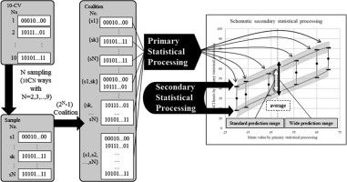
We regarded a range between the 2 mean values obtained in the secondary statistical processing as the standard estimated range. We also generated a wide estimated range from the maximal and minimal values of the 6 values in the secondary statistical processing for the maximal upper limit and the minimal limit, respectively. If the estimation range limits were less than 0 or greater than 100, they were replaced with 0 or 100, respectively. Various mathematical distribution models can be used for the curve fitting method. In the primary and secondary statistical processing, we used 3 types of distribution; the normal distribution, the Poisson distribution, and the binominal distribution. We thus obtained a total of 9 standard estimated ranges and 9 wide estimated ranges. Figure 2 provides a schematic explanation of the process for making the estimation ranges from N samples.
Judgement: We scored the estimation success rates if the range by G-EPOC included the true mean of all 10 samples in the simulation dataset for all combinations with N assigned as 2, 3, 4, …, and 9, with which the numbers of combinations were 10C2 = 45, 10C3 = 120, 10C4 = 210, …, and 10C9 = 10, respectively. Finally, we selected the best series of statistical processing for each of N samples according to the following conditions: (1) more than 95% of the number rate of the successful estimated ranges, and (2) the narrowest averaged estimated range width.
Figure 1
Distribution of the scores of 10 samples in the simulation dataset. We set the distribution to follow the sigmoid function 1/(1 + exp (–αx)) under α = 1.28 and x = 0.05 to 0.95 with 0.1 as the increment, adjusting to the conditions for 100 and 0 for the maximal and minimal scores, respectively
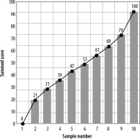
Figure 2
The process for making the estimation ranges from N samples. After we made (2N – 1) possible coalitions from N samples of 10 results of 10-CV, we applied them to 3 types of probability distribution fitting and then 3 types of generalized linear model fitting as the secondary processing. We then obtained the standard estimated range and the wide estimated range from the upper, mean, and lower limits of 95% CIs with N assigned as 2 to 9
Practical test
In the second test for G-EPOC, we assessed the ability of G-EPOC to estimate the mean accuracy of 10-CV validating the practical datasets as follows:
Patients: As the appendicitis group, we enrolled a total of 485 patients with appendicitis, who underwent a contrast-enhanced computed tomography examination (CECT) due to acute abdomen in the period from January 2010 to March 2019 (male/female, 269/216; age range/average, 6-98/38.5 years). They were diagnosed based on 1-mm slice thickness CT as well as clinical findings. The following CT criteria were used for diagnosing appendicitis [19-22]: appendix diameter of more than 6 mm, appendiceal wall enhancement, presence of appendicoliths, periappendiceal fat stranding, and concomitant abscess.
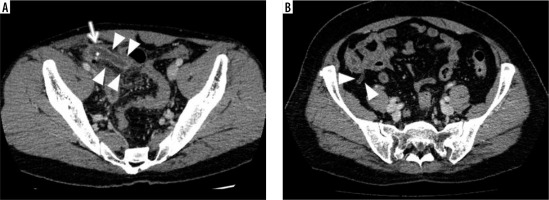
For the control group, we randomly selected 485 patients who underwent a CECT due to acute abdomen enrolled backward from March 2019 to December 2016, in order to include the same number of patients as in the appendicitis group (male/female, 245/240; age range/average, 13-97/64.2 years). Their results were negative for appendicitis but might be positive for other acute abdominal disorders. Their detailed diagnoses are not provided here because they were too varied to describe and they were not relevant to the present study. Figure 3 shows representative examples of CT images in the appendicitis and control groups.
Computed tomography: Multidetector row CT was performed using clinical CT units (Aquilion CX, Aquilion 64, and Aquilion ONE, Canon Medical Systems, Ohtawara, Japan; SOMATOM Definition Flash, Siemens Healthineers, Erlangen, Germany; Discovery CT750 HD; GE Healthcare, Chicago, IL). CT images were generated using a body window algorithm, a 220-500-mm field of view (FOV), 512 × 512 matrix, and a 1-mm slice. The iodine contrast agent was intravenously injected according to the following protocols: iodine volume per weight, 600 mgI/kg; Contrast agent, iopamidol (300 mgI/ml), iopamidol (370 mgI/ml), iohexol (300 mgI/ml), iohexol (350 mgI/ml), or iomeprol (300 mgI/ml); injection speed, 5 to 2.0 ml/s bolus injection; start of helical scanning, 70 to 230 s after the injection of the contrast. Decreased volumes were adopted in cases of the patient’s declining renal function based on the physician’s request.
Extraction of positive and negative image data: We chose 20,690 positive images that included any cross-sections of the enlarged and enhanced appendix indicating appendicitis extracted from the patients with appendicitis. We used multiple slices from the same subject as described previously [4,6,14].
We extracted 297,636 negative images from the control group, covering the entire abdominal areas.
Practical dataset preparation: We prepared five datasets of 124, 250, 374, 500, and 624 pairs of the randomly extracted positive and negative CT images from both the appendicitis group and control group, respectively. The sizes of five datasets were adjusted to meet 100, 200, 300, 400, and 500 pairs of the training images with the ratio of 1/10, 1/10, and 8/10 for the testing, verification, and training image numbers for each of the datasets. We regularized the sampling size based on the size of the training images instead of the total sample images because 10-CV could be more sensitive to the former than the latter [14]. We did not use all the 20,690 positive images because we realized that a 10-CV using 20,690 positive images provided more than 90% of the mean accuracy, which had a ceiling effect and was thus not suitable for the current test.
Image data processing: We used one of the representative DL convolutional neural networks, AlexNet, which was designed by Alex Krizhevsky and won the Image-Net Large-Scale Visual Recognition Challenge in 2012, in the pre-trained state with over a million images from the ImageNet database (ImageNet. http://www.image-net.org) [23]. We adopted the transfer learning method for training AlexNet as described previously [4,6,14]. The AlexNet that we used in this study did not support the Digital Imaging and Communications in Medicine (DICOM) format. Using the free software program Fiji (https://imagej.net/Fiji), we converted these images from the DICOM format into Portable Network Graphics (PNG) with 16-bits and 227 × 227 pixels of the image size with adjustment of the brightness and contrast of the original DICOM image by using the look-up-table (LUT) function in the Fiji program.
10-CVs for validating AlexNet enabled for the task of detecting appendicitis: We applied 10-CV to the above-mentioned 5 practical datasets as follows. (1) The dataset was split into 10 equal parts. (2) The ratio of the data was set as 1/10, 1/10, and 8/10 for the testing, validation, and training image numbers, respectively. (3) AlexNet was trained with the training images. (4) AlexNet was validated with the validation images to prevent over-training. (5) AlexNet was tested with the testing images to evaluate its judgment ability. (6) This process was repeated 10 times, each time with a different 3 parts of testing, validation, and training datasets. (7) The mean accuracy was determined by averaging the 10 results of the testing.
As the referential standard, we determined the mean accuracies and the 95%CI ranges with the t-distribution calculated from the result datasets of the 10-CV in each of the 5 practical datasets.
Testing and judgment: We changed each of the result datasets to the Boolean expression consisting of 0 points for false and 1 point for true. We applied each of the N samples extracted from the result datasets of the 10-CV in each of the 5 practical datasets to the best G-EPOC processing determined in the simulation test as described above. We scored the number rates of the estimation range, which successfully included each of the mean accuracies of 10-CVs of the 5 practical datasets for all combinations with N assigned as 2 to 9. We then recorded the successful estimation rates, the average of the successful estimated range widths, and the averages of upper and lower limits of the successful estimated ranges. We plotted the mean accuracy line of the 5 practical datasets in conjunction with the averaged estimation range areas (ERAs) whose upper and lower boundary lines were the averaged upper and lower limits of the successful estimated ranges by G-EPOC.
Figure 3
Representative examples of CT images in the appendicitis and control groups. A) Contrast-enhanced abdominal CT of a 32-year-old male in the appendicitis group shows an enlarged appendix with thickened wall enhancement (arrowheads) in conjunction with fluid and an appendicolith inside (arrow) at the right lower quadrant in the abdomen. B) The CECT of a 54-year-old female in the control group shows a normal gas-filled appendix with non-enhanced thin wall (arrowheads) at the apex of the cecum
Test using the first N sampling
In the third test for G-EPOC, we estimated the ability of G-EPOC in the following pragmatic situation:
In a pragmatic situation, G-EPOC users do not necessarily calculate all combinations with a given N, which is assigned as 2 to 9, out of the result datasets of 10-CV. Instead, they may stop performing 10-CV halfway and use the first N of the result datasets of 10-CV for making the estimation range. Moreover, they may regard the midpoint of the estimation range by G-EPOC as a surrogate estimated value for the mean accuracy of 10-CV. Assuming such a case, we made the following judgment: We obtained the midpoints between the upper and lower limits of the estimation range in each of the first sampling trial with N assigned as 2 to 9. We recorded the number N as successfully estimated by G-EPOC when the 95% CI ranges with the t-distribution of the 5 practical datasets included the midpoints provided by G-EPOC. We plotted the mean accuracy line and the 95% CI range areas with the t-distribution of the 5 practical datasets, plus the midpoint lines afforded by G-EPOC from the result datasets of the 10-CV in each of the 5 practical datasets for the first N sampling. We also evaluated the expected time-saving (%) of the first N of the result datasets of 10-CV calculated from (C – (A + B))/C, where A was equal to the processing time (s) of the first N sampling of G-EPOC, B was equal to the acquisition time (s) of the first N sampling of the practical datasets of 10-CV, and C was equal to the acquisition time (s) of all 10 result datasets of 10-CV.
Other conditions
Hardware and software for computational processing
We used a custom-built image processing computer (TEGARA Corp., Hamamatsu, Japan) containing a Quadro P2000 5 GB graphics processing unit (Nvidia Corp., Santa Clara, CA), an Intel Xeon E5-2680v4 2.40 GHz processor (Intel Corp.), 1.0 TB of hard disk space, and 64 GB of RAM. We used MATLAB software (ver. 2018b; MathWorks Inc., Natick, MA) for all statistical computational processing. The AlexNet algorithm that we used was distributed as add-on software of MATLAB.
Results
Simulation test
For the best series of the primary and secondary statistical processing, we identified the binominal and binominal distribution models for N as 2, the normal and binominal distribution models for N as 3 to 8, and the Poisson and normal distribution models for N as 9. We adopted the wide estimated ranges for N as 2 to 8 and the standard estimated range for N as 9. As a result, we obtained 98% to 100% successful estimation rates with all numbers of sampling out of 10 samples in the simulation dataset. When the N was increased from 2 to 9, the averaged widths of the successful estimated ranges narrowed from 88.8% to 13.6%. Table 1 summarizes the results of the simulation test.
Table 1
Results of the simulation test
Practical test
We obtained 98% to 100% successful estimation rates for all numbers of sampling in the 5 practical datasets by applying those datasets to the best series of the successful estimation processing obtained in the simulation test. Table 2 shows the mean accuracies of the 5 practical datasets, the averages of those estimated range widths, and the averages of the upper and lower limits of those estimated ranges by G-EPOC. Figure 4 illustrates the mean accuracy line of the 5 practical datasets and ERAs with the N assigned as 2 to 9 by G-EPOC. The mean accuracy line is completely covered by ERAs by G-EPOC. The upper and lower limits of the ERAs approached the mean accuracies of 10-CV results as the number of samplings increased.
Figure 4
The mean accuracy line for 5 practical datasets and the estimation range areas (ERAs) by G-EPOC. The mean accuracy line is completely covered by ERAs by G-EPOC
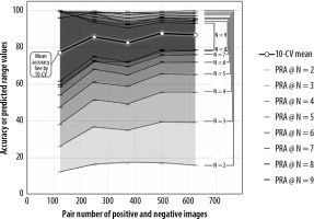
Table 2
Results of the practical test
Test using the first N sampling
The midpoints of the ranges between the upper and lower limits of the first N sampling with the N assigned as 8 and 9 by G-EPOC were included by the 95% CI range with the t-distribution for all 5 practical datasets. However, some of the midpoints with the N assigned as 5 to 7 and all of those with the N assigned as 2 to 4 missed the 95% CI range with the t-distribution. Figure 5 provides the mean accuracy line and the 95% CI range areas with the t-distribution calculated from the 5 practical datasets, plus the midpoint lines from the result datasets of the 10-CV in each of the 5 practical datasets for the first N sampling by G-EPOC with the N assigned as 2 to 9.
Figure 5
The mean accuracy line and 95% CI range areas with t-distribution of the 5 practical datasets, and the midpoint lines in each for the first N sampling trial. The midpoints of between the upper and lower limits of the first sampling by G-EPOC with 8 and 9 as the N were included by the range of 95% CI with the t-distribution of all 5 practical datasets. However, some of the midpoints with the N assigned as 5 to 7 and all of those with the N assigned as 2 to 4 missed the 95% CI range with the t-distribution
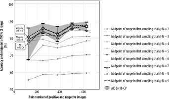
Tables 4-6 show the processing time (sec) of the first N sampling of G-EPOC, the acquisition time (sec) of the first N sampling of the practical datasets including the total 10 result datasets of 10-CV, and the expected time-saving (%) of the first N of the result datasets of 10-CV. The acquisition times of the first N sampling of the practical datasets ranged from 363 to 8118 sec, whereas the processing time of G-EPOC ranged from 0.61 to 3.64 sec. The expected time-saving (%) was thus approximately 10% per one result of 10-CV skipped.
Table 3
Results of the random dataset test
Table 4
Acquisition time (sec) of the first N sampling of G-EPOC
Table 5
Acquisition time (s) of the first N sampling of the practical datasets
Table 6
Expected time-saving (%) of the first N of the result datasets of 10-CV
Discussion
In the simulation test, we obtained 98% to 100% successful estimation rates with all numbers of sampling out of 10 samples in the simulation dataset. Because the possible summed scores in one sample thus ranged from 0 to 100, which presumed the extreme case, our present analyses clarified that G-EPOC could estimate the range of the mean accuracy by any situation of 10-CV using less than 10 results at the rates of more than 95%. We adopted the standard or wide ranges calculated by the primary and secondary statistical processing using the binominal, normal, or Poisson distribution, although the mathematical appropriateness for the current processing was not clarified.
In the practical test, we obtained 98% to 100% successful estimation rates for all numbers of sampling in the 5 practical datasets by G-EPOC using the best series of the successful estimation processing obtained in the simulation test. Our results confirmed that G-EPOC could estimate the range of the mean accuracy by any situation of 10-CV using less than 10 results in a practical situation. Figure 4 demonstrates that the upper and lower limits of the estimation range of G-EPOC approached the mean accuracies of 10-CV results as the number of samplings increased. However, the estimation ranges of G-EPOC are apparently wider compared to the 95% CI ranges of 10-CV results with t-distribution. This is a compensatory trade-off for accomplishing over 95% accuracy.
We assessed the pragmatic use of G-EPOC; i.e., the midpoint of the estimation range with the first N sampling as a surrogate estimated value. As a result, the midpoints of the estimation range with the N assigned as 8 and 9 were placed inside of the 95%CI range with the t-distribution of the 5 practical datasets. Therefore, G-EPOC might be effectively used with the N assigned as 8 or 9, in which approximately 10% to 20% would be spared because about 10% of time-saving per one result of 10-CV was confirmed.
G-EPOC has been proposed as an option for the selection of the optimal K value in K-CV; i.e., it is possible to make an almost perfect estimation even if the training and validating DL is repeated fewer than 10 times in 10-CV.Although G-EPOC does not necessarily have a direct clinical contribution, G-EPOC as an alternative to 10-CV will save time and computer resources in the process of developing the CADDELAC system. G-EPOC might be also effective for the early introduction of the CADDELAC system for clinical applications.
There are some limitations to this study. Narrower range estimations should be achieved with further investigations, although we suggested the pragmatic use of the midpoint of the estimation range with the first N sampling. The G-EPOC findings obtained herein are empirical results, and there is still no mathematical or statistical basis to support them. Further research is required.
Conclusions
G-EPOC demonstrated over 95% successful estimation for the accuracy determined by 10-CV, using less than 10 results of 10-CV, which was confirmed by the datasets obtained from the real detection task of appendicitis on CT by AlexNet. Our series will help lessen the consumption of time and computer resources in the development of computer-based diagnoses in medical imaging.


