Introduction
Many factors contribute to diabetic foot ulcers (DFUs), including exercise, diet, and insulin therapy. A diabetic patient’s foot soles may have open lesions or lacerations due to these ulcers. As of 2019, approximately 463 million people were living with diabetes worldwide [1]. There are 9.1 million to 26.1 million diabetic patients in the world who suffer from DFUs each year; 15 to 25% of them experience the condition at some point in their lives [2]. The complexity of DFU diagnosis and treatment results in almost a million diabetics losing a limb each year.
Several factors, including poor blood circulation, hyperglycaemia, nerve damage, and inflamed feet, cause foot ulcers. Other risk factors include inadequate hygiene, improper clipping of toenails, eye disease, any kind of heart disease, kidney failure, excess fat or obesity, and consumption of tobacco or alcohol.
Initial symptoms of DFUs encompass foot drainage, pain, paralysis, peculiar irritation, oedema, erythema, and odorous discharge. The most visible sign of significant DFUs is the presence of black tissue surrounding the lesion due to insufficient blood supply to the ulcer’s vicinity. Infections can lead to partial or complete tissue death in this region, although it may take a while before ulcers become infected [3]. Additionally, weeks or sometimes months are required for DFUs to heal, with reappearance rates reaching 40% after one year, 60% after three years, and 65% after five years. Alarmingly, 14-24% of cases eventually necessitate lower extremity amputation [4].
The early detection of DFUs is crucial for effective treatment. If identified promptly, methods such as foot bathing, maintaining clean and dry skin around the ulcer, enzyme therapies, and bandages with calcium alginates can prevent growth of bacteria. However, as the condition worsens, severe surgery may become necessary for recovery or removal of the ulcer [5]. DFU diagnosis typically involves testing for secondary infections, X-rays to assess bone involvement, angiography, and other diagnostic techniques.
To establish an accurate diagnosis, comprehensive medical data analysis is essential. Traditional diagnostic methods can be labour-intensive and prone to human error. Utilizing computer-assisted diagnostic procedures can enhance efficiency while reducing costs. Recent advances in mobile and ubiquitous health devices play a significant role in managing diabetes and its complications by monitoring inflammation and detrimental foot pressure [6]. Sensors, capable of detecting various types of chemical, physical and biological signals, offer a means to identify and record these captured signals. These sensors, initially developed for industrial applications, have found new applications in healthcare [7].
Medical imaging [8-11] is a cornerstone for diagnosing various patient conditions in today’s digital healthcare landscape. The efficacy of traditional classification of machine learning (ML) and deep learning (DL) methods in medical imaging depends heavily on type of feature selection and extraction techniques, which are sensitive to the shape, size, and colour of the captured images. Researchers have achieved high accuracy in DFU detection using ML and convolutional neural network (CNN) techniques, although there is still room for broader real-world applications [12].
Early identification of DFUs in contemporary healthcare systems involves continuous surveillance and management. To inform treatment plans, diabetic foot specialists conduct thorough examinations of DFUs along with additional diagnostic tests such as magnetic resonance imaging (MRI), X-ray and computed tomography (CT) scans [13]. However, to conduct and verify these tests, appropriate time, with frequent visits to hospitals and and specialists, is required, which can potentially worsen the disease before intervention. It underscores the prominence of a computer-assisted diagnosis system capable of identifying DFUs before they become visually apparent [14].
The main purpose of this study was to detect foot ulcers using creation of a pre-processed dataset by applying edge detection and segmentation. Then for prediction a DL model was applied and the performance of the proposed model was compared. The main contributions of this study are as follows:
The objective of this study was to design and implement a comprehensive machine learning algorithm that can accurately and reliably differentiate between instances of diabetic foot ulcers (DFU) and normal foot conditions using thermal images.
The development of a model using a plantar thermogram database facilitates early diagnosis by detecting elevated plantar temperatures before the occurrence of a DFU. The thermal measurements exhibit reduced susceptibility to the influence of the surrounding circumstances.
To enhance the quality of the outcomes, it is recommended that canny edge detection and watershed segmentation be used on images and a pre-processed dataset be created. This combination enables one to obain more clearly recorded local and global texture and shape information.
The performances of the evaluated models are compared with some existing studies.
A critical aspect of the concept is the ability to do real-time testing.
The rest of the paper is divided into various sections. Section 2 describes some related studies and their limitations. The techniques used to design a pre-processed dataset for better prediction is defined in section 3. Section 4 illustrates the proposed model, algorithm and mathematical equations used. Section 5 gives an overview of simulation software and performance metrics evaluation. Finally, section 6 presents the conclusion and future scope of research.
Related work
A comprehensive review of relevant literature was undertaken to learn about the current body of research. The following content summarizes the scholarly articles about the relevant research.
In one study, the authors conducted a widespread examination of the existing literature on the utilization of artificial intelligence (AI) in monitoring DFUs [15]. The study discussed the advantages of these techniques and highlighted the challenges associated with integrating them into a functional and dependable structure for effective management of remote patients. This research examines the imaging methods and optical sensors used to detect diabetic foot ulcers. The investigation takes into account the characteristics of the sensors as well as the physiological aspects of the patient. The data source supported various monitoring strategies, which imposed constraints on AI technologies.
In another study [13], a unique CNN model was created to classify healthy and abnormal skin automatically. This CNN was trained using a dataset of 754 colour photographs of DFUs and normal skin samples obtained from the diabetes centre at Nasiriyah Hospital. An expert in DFU manually annotated the database in order to create the ML model. The region of interest (ROI) dimensions were adjusted to 224 × 224 pixels. This modification resulted in a substantial area encompassing the ulcer, including crucial tissues from the normal and DFU categories. A trained expert then proceeded to annotate the clipped patches. The researchers used the DFU_QUTNet classifier to evaluate the performance of their model. The acquired F1-score was 93.24%. Additionally, they integrated network characteristics with an support vector machine (SVM) classifier, resulting in an improved performance of 94.5%.
Researchers [16] proposed the use of a non-invasive photonic-based apparatus as a potential treatment modality for addressing DFUs in patients diagnosed with problem of diabetes. The apparatus used the principles of hyperspectral and thermal imaging to evaluate the condition of a foot ulcer. The biomarkers of oxyhaemoglobin and deoxyhaemoglobin were estimated using photonic based imaging. By using super-resolution methods, the apparatus underwent enhancements via the incorporation of signal processing technologies that use deep learning algorithms to increase pixel accuracy and reduce noise.
In a study [17], the authors proposed using a specialized network called Dfu_SPNet, which is constructed using parallel stacked convolution layers, to classify the data of ulcer images. Dfu_SPNet used parallel convolution layers with three distinct kernel sizes in the context of feature abstractions. Dfu_SPNet achieved a superior performance compared to the current state-of-the-art results, as shown by its area under the curve (AUC) score of 97.4%. This notable improvement was seen after training the Dfu_SPNet model on the dataset, using the stochastic gradient descent (SGD) optimizer with a learning rate of 1e-2.
In a study [18], DFU classification using CNN was performed, and the researchers used RGB, i.e. 3 channel images, and corresponding information of texture as inputs for the proposed CNN model. The researchers found that the suggested framework exhibits superior classification performance compared to conventional RGB-based CNN models. The study’s first phase involved using the mapped binary pattern approach to gather the texture information of the RGB image. The mapped image generated from the ulcer texture information was used in the second step to aid in identifying DFUs. The CNN received a tensor input that is called a fused image, which is composed of a linear combination of the RGB and mapped binary pattern. The model achieved an F1 score of 95.2%.
In a further investigation [19], the authors used a dataset consisting of 50 thermograms captured at a distance of one foot. The classification task was carried out using a traditional machine-learning methodology. The intensity values of thermograms from both normal and diabetic feet were used to generate grey texture features. These features were then utilized as the input for the classifier model SVM. The accuracy of classification was determined to be 96.42%.
In a study [20], the authors used 33 thermographic images of the plantar foot region, including persons without any medical conditions and those diagnosed with type 2 diabetes. The decomposition of foot images was done using the discrete wavelet transform (DWT) with techniques of higher order spectra (HOS). The generated decomposed images were further used to find different texture and entropy attributes. The SVM classifier achieved a 81.81% sensitivity score, 89.39% accuracy, and a specificity of 96.97% based on a limited set of five features.
The authors of another study [21] devised an innovative skin tele-monitoring system that utilizes a smartphone to improve the medical diagnosis and decision-making process in assessing DFU tissue. In order to accurately identify tissues and label the ground facts, a dataset consisting of 219 photos was used. A graphical interface was also developed based on the super pixel segmentation technique. The system’s method included a thorough examination of DFU, including automated ulcer segmentation and categorization. The retrieved super pixels serve as the training input for the deep neural network, and classification at the patch level was performed. The model under consideration had an accuracy of 92.68% and a DICE score of 75.74%. An alternative methodology [22] extracted features from the CNN model known as Densenet201. These features were then inputted into a SVM classifier to facilitate the diagnosis of DFUs.
Several other studies have examined the location of infection in conjunction with its categorization. In a study [23], a CNN architecture consisting of 16 layers was presented for the purpose of classifying infection/ischemia models. The process included extracting deep features, which were then used as the input for a range of machine learning classifiers in order to assess the performance of the model evaluation metrics. In addition, the researchers used gradient-weighted class activation mapping (Grad-CAM) to visually represent the prominent characteristics of an infected zone, hence facilitating a more comprehensive interpretation after the classification process. The photos were inputted into a YOLOv2-DFU network to identify and localize affected regions. The suggested model demonstrated an accuracy of 99% for infection classification and 97% for ischemia classification. In order to identify and pinpoint areas of the foot that are affected by unhealthy conditions, the researchers achieved an intersection over union (IOU) score of 0.98 for ischemia and 0.97 for infection.
In other research [24], a thorough examination of model scaling was undertaken, revealing that the meticulous optimization of network breadth, depth, and resolution may achieve performance enhancements. Based on the result above, a unique scaling approach was proposed, which used a simple but very effective compound coefficient to uniformly scale all three parameters. A baseline network was developed using neural architecture and then expanded to generate the EfficientNets series of models. These models show superior performance compared to previous convolutional neural networks (ConvNets) in terms of effectiveness and accuracy. Additionally, they exhibited the advantages of smaller size and quicker inference speed. Notably, the EfficientNets achieved an accuracy rate of 84.3% on the ImageNet dataset.
Furthermore, there is a limited body of research that has used thermal imaging of the foot, since the majority of studies have relied on visual foot images that are vulnerable to fluctuations in the surrounding environment. In order to address these constraints, we have devised a dependable and entirely automated computer-aided design compatible model based on DL techniques for the purpose of diagnosing DFUs. Thermal imaging was selected as the preferred method for monitoring the distribution of temperature over the foot, with the aim of aiding in the timely detection of DFUs. In addition, the thermal images exhibit reduced susceptibility to the influence of the surrounding environment. In addition, before testing the model for better predictions and accuracy the pre-processing techniques canny edge detection and watershed segmentation were applied and a pre-processed dataset was created. Canny edge detection highlights the edges in an image, providing important features for subsequent analysis. These edges can capture important structures and boundaries in the image, which can be useful for classification tasks [8]. Edge detection can also help reduce noise in the image by emphasizing only the most significant edges. This can also improve the quality of the input data for classification algorithms, leading to more accurate results. Watershed segmentation can partition the image into regions based on gradients and intensities, effectively separating different objects or regions of interest [25]. This segmentation can help isolate individual objects or areas within the image, making it easier for the classifier to focus on relevant features.
Material and methods
Dataset
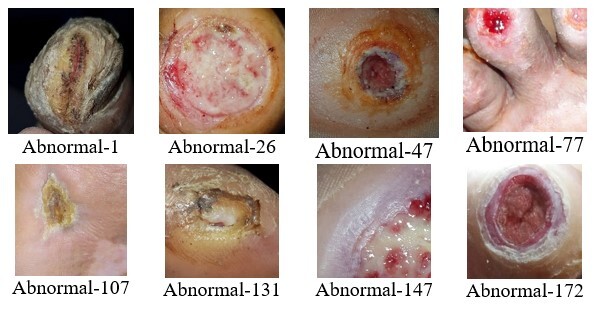
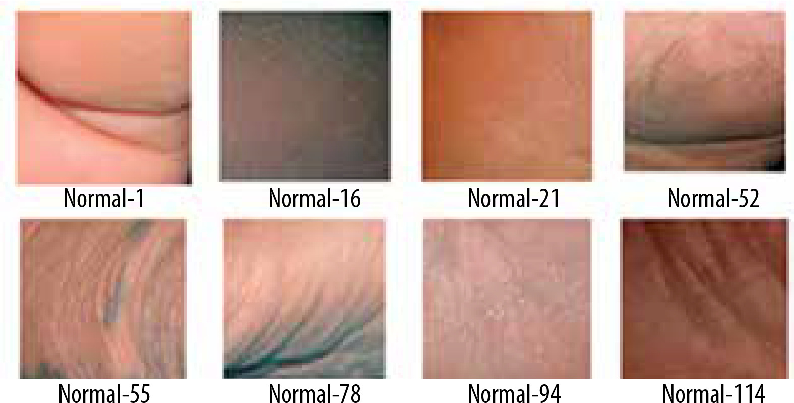
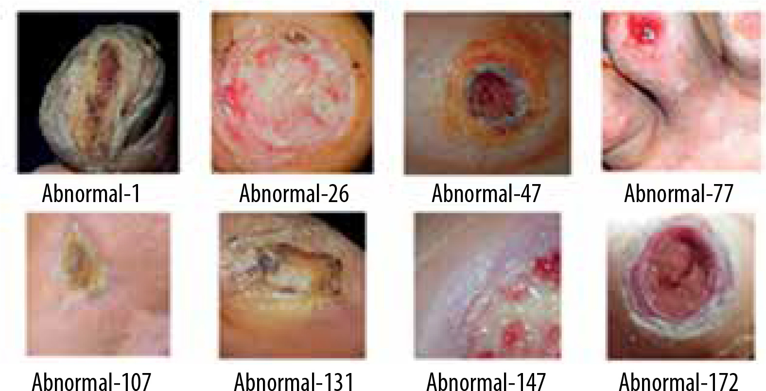
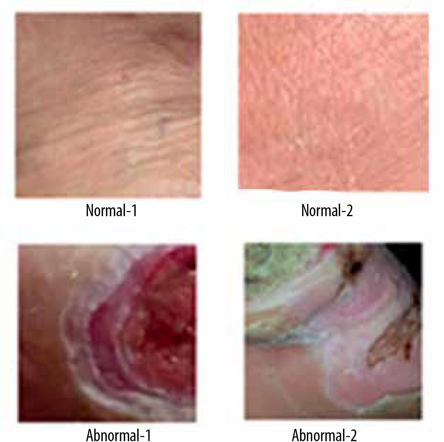
A thermogram image dataset was used for this study [14]. The dataset consists of two type of images – normal and ulcer. In total, 1055 images are present in the dataset; among these images, 543 are normal and the rest are of ulcers. A sample of normal feet images from dataset is shown in Figure 1, while Figure 2 shows sample images of abnormal feet from the dataset. Both types of files are organized in separate folders named normal and ulcer respectively and labelled with numbering.
Canny edge detection
The images in the dataset were transformed using the canny edge detection technique. Canny edge detection is a technique widely used in computer vision for detecting edges in images. Since its creation in 1986 by John F. Canny, it has evolved into one of the industry norms for edge detection. The basic steps involved in the process are as follows: The input image is smoothed, Eq. 1 represents the equation of the 2D Gaussian function, and edges of the image are detected using the Sobel filter. The Sobel operator calculates the gradient Gx in the x direction and Gy in the y direction using the kernel given in Eq. 2 and 3. After this, suppression of type non-max is applied and the local maximum pixels in the gradient direction are reserved; the rest of the pixels are blocked. Eq. 4 and Eq. 5 represent the gradient magnitude and gradient direction respectively. The thresholding is applied to remove the pixels which are less than a certain threshold value and pixels are considered if above a certain threshold value to remove the edges that could be formed due to noise. Finally, hysteresis tracking is applied with the two thresholds Thigh and Tlow to classify pixels as strong, weak and no edge [8, 26].
Where F(x, y) is a Gaussian kernel at position (x,y), standard deviation is represented as σ of the Gaussian distribution, e is the base for the logarithm, and the coordinates are x and y in the Gaussian kernel.
Where GM(x, y) represents gradient magnitude and θ(x, y) represents gradient direction.
Watershed segmentation
The watershed algorithm is a method of separating images that relies on watershed transformation. The segmentation method relies on the relative similarity of neighbouring pixels in the image as a crucial point of reference for linking pixels with similar spatial coordinates and grey values.
The watershed method uses topographic information to partition an image into distinct parts. The method considers the image as a topographic surface and uses pixel intensity to locate catchment basins. Starting locations are designated local minima, and catchment basins are filled with colours until the object’s limits are reached. The segmentation process gives distinct colours to certain areas, facilitating the identification of objects and the study of images [25, 27].
The whole procedure of the watershed algorithm may be succinctly outlined via the following steps:
Placement of marker – the watershed segmentation involves strategically placing markers on the local minima, the lowest points in the image. These markers serve as the initial reference points for the subsequent flooding process.
Flooding – it is a key technique in the watershed method, involves saturating the image with various colours, starting from the markers. This colour dispersion gradually fills the catchment basins, extending beyond the borders of the objects or regions depicted in the image.
Formation of catchment basins – the process of colour dispersion leads to the progressive filling of catchment basins, resulting in the segmentation of the image. The segments or areas obtained are allocated distinct colours, which may be used to distinguish various items or characteristics within the image.
Identification of boundaries – the watershed method employs delineating borders between distinct coloured sections to ascertain the presence of objects or regions within the image. The segmentation obtained may be used for many applications, such as object identification, image analysis, and feature extraction.
Data augmentation
In order to operate efficiently, deep learning model requires a substantial amount of labelled training data. In addition, gathering a large amount of medical data is costly and difficult. In order to enhance the performance of the deep learning model and avoid the problem of overfitting, the data augmentation technique is used. Various image processing methods are used for data augmentation to achieve the intended outcomes, such as resizing, rotation, and translation.
Resizing – Through this dimensions of the image are changed. Let I0 be the original image with dimensions (H0, Wo, C0) , where H0 is height, Wo is width and C0 is number of channels. Resizing is calculated by Eq. 6.
Where
Random Rotation – Let I0 be the original image. Random rotation is calculated by Eq. 7.
Where θ is a random rotation angle.
Random Translation – Let I0 be the original image. Random rotation is calculated by Eq. 8.
Where tx, ty are random translation amounts in the horizontal and vertical directions respectively.
Random Flip – Let I0 be the original image. Random flipping is calculated by Eq. 9. The flip operation can be horizontal or vertical, which will be chosen randomly.
Gaussian Noise – Let I0 be the original image. Gaussian noise is calculated by Eq. 10.
Where μ is the mean and σ is standard deviation of the Gaussian distribution.
Random Contrast – Let I0 be the original image. Random contrast is calculated by Eq. 11.
Where Cf represents the random contrast factor.
Proposed model
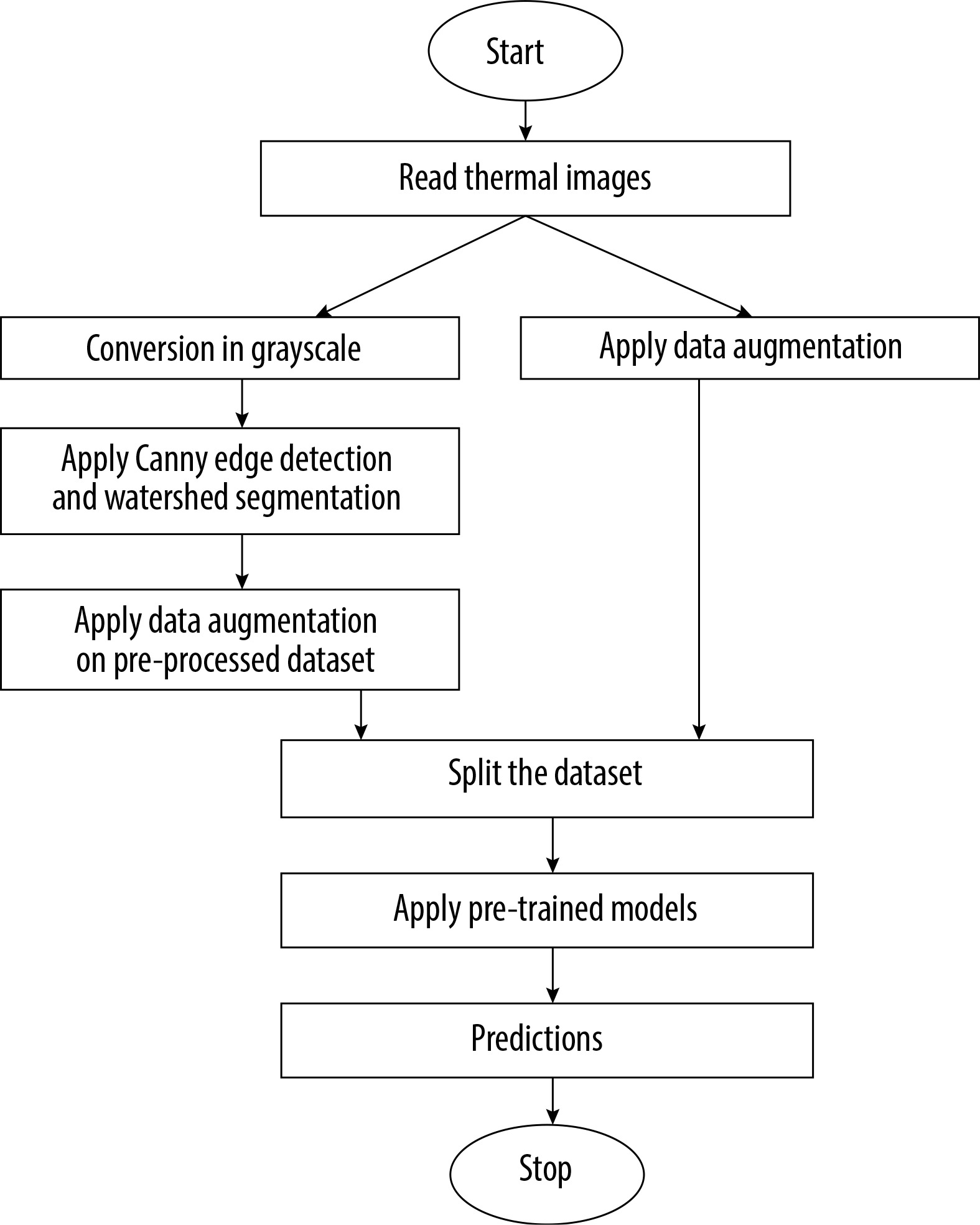
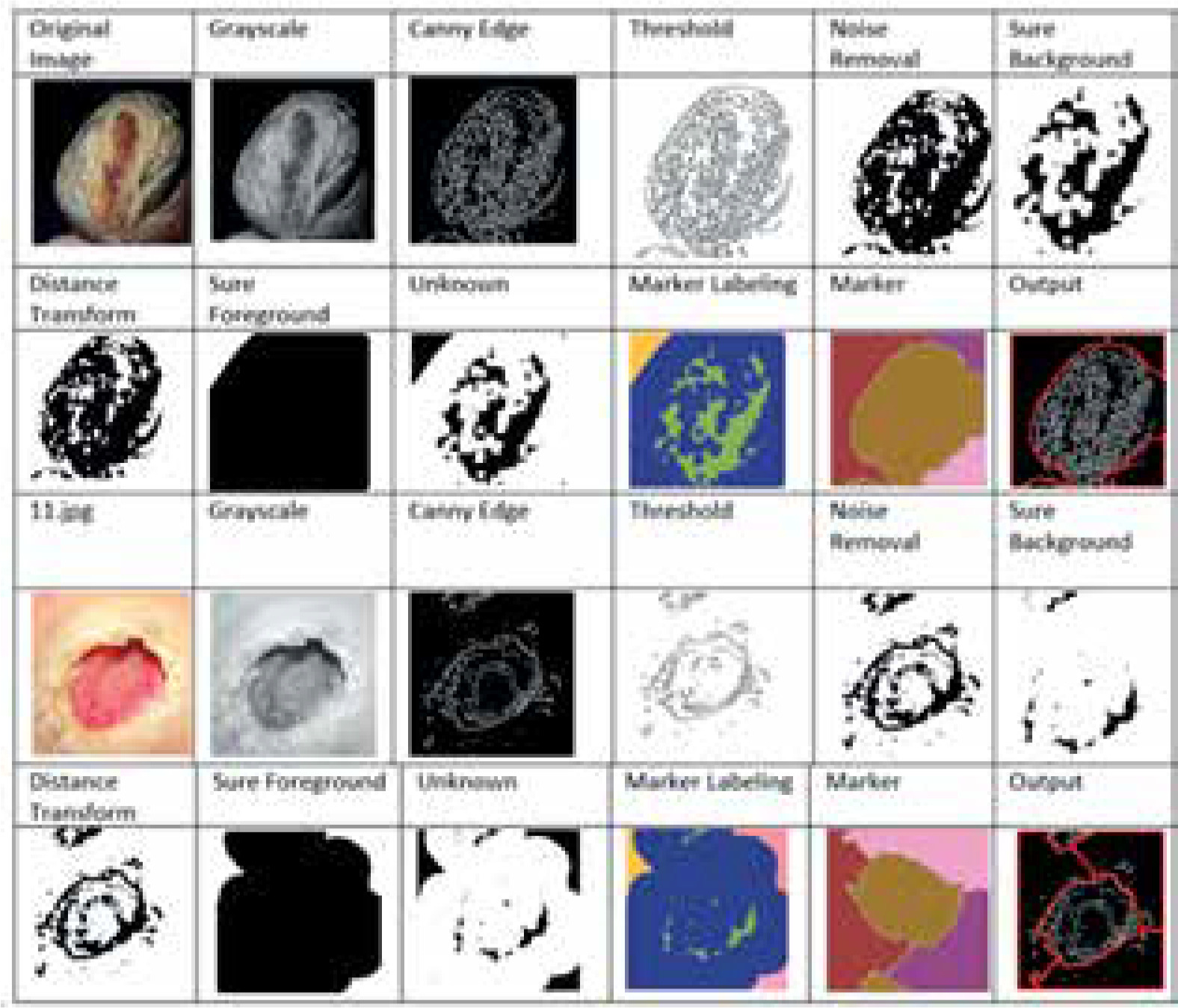
This section provides an overview of the deep learning models used for the prediction of foot ulcer instances. The model is trained using a regression classifier utilising a scaled and filtered image dataset, after feature extraction using pre-trained models and filters. Figure 3 displays the block diagram of the suggested model, whereas Algorithm 1 illustrates the significant processes involved in the proposed model. The approach under consideration was assessed using the whole dataset, including both normal and diseased images. In the proposed method a new dataset is created by applying the canny edge detection and watershed segmentation on the images present in the dataset. In the first step canny edge detection is applied to all the images of the normal category and the abnormal category. After edge detection the watershed marker segmentation is applied on the images obtained after edge detection. All the converted images are subsequently stored in the two folders converted_normal and converted_abnormal. Figure 4 shows an example image obtained after each step of the edge detection and segmentation. The output image obtained is the image of the new dataset. After creation of the new dataset, the data augmentation with six methods is applied to accomplish two goals – one to increase the size of the dataset for training of the models and another to balance the dataset as 543 images are normal and 512 are abnormal.
The following part provides a comprehensive analysis of the training, testing, and other factors. The classification model utilises the Adam optimizer, which is based on SGD. The primary differentiating factor between Adam optimizers and SGD is in their updating processes. SGD calculates gradients as per a single training instance randomly to update the model’s parameters. In contrast, Adam combines the advantages of adaptive learning rates and estimates of first- and second-order moments of the gradients. This leads to more effective and efficient parameter updates. The learning rate in the Adam optimizer is adjusted dynamically during training by using averages of the parameters. Eq. 12 illustrates the loss function. Table 1 illustrates the detailed parameters of the model.
Table 1
Parameters of the model
Where, at time t , Gt represents the gradient of the loss function, the gradient operator is represented by ∇ , θt – model parameters at time t , FL – loss function and Dtrain – training data. The first and second moments of the gradients are initialized by 0 and represented as M0 , V0 = 0. Eq. 13 is used to update the first moment.
Where γ1 represents the exponential decay rate. The second moment estimate is updated using Eq. 14.
Where γ2 represents the exponential decay rate. Eq. 15 and 16 are used for calculation of bias.
Model parameters are updated using Eq. 17
Where learning rate is represented by α and τ is a small constant.
In the proposed models sparse categorical cross entropy is used to measure the divergence between the predicted probabilities and actual probabilities of the dataset. Eq. 18 shows the cross entropy for single training. Eq. 19 shows the average cross-entropy loss over the entire dataset.
Where Li is the loss for the ith training sample, pi,yi is the logit corresponding to class j for the ith training sample. yi is the true label for the ith training sample and C is the total number of classes.
Where N is the total number of samples.
Algorithm 1:
Input – 1055 thermal images.
Output – Prediction as normal or abnormal ulcer feet.
Begin:
Load dataset with normal (D_normal) and abnormal (D_abnormal) images
Convert to grayscale
DC_normal, DC_abnormal=canny_edge_detection(D_normal, D_abnormal)
DS_normal, DS_abnormal=watershed(DC_normal, DC_abnormal)
X_augmented=data_augmentation(DC) // Combined dataset
Train_X, Val_X=Split dataset for training and validation
Apply Resnet50 and EfficientNetB0 pre-trained model
Compile the model using the Adam optimizer and sparse categorical cross entropy as the loss function
Train the model for 20 epochs and print the classification report
Test model on real data using Test_y. //Test_y contains images taken randomly from clinics
Repeat steps 7 to 10 without edge detection and segmentation.
End.
Results and discussion
The model was simulated using Python 3.x , with a Jupyter notebook on a system with primary memory of 16 GB and GPU of 4 GB, 8th Generation Intel PC [28]. For training and testing of the model an open source dataset of thermal images was utilized. The deep learning models Resnet50 and EfficientNetB0 were used for the analysis. Training of the models was done in two phases. In the first phase both models were trained and validated using the original dataset of thermal images and performance metrics were noted down. In the second phase the models were trained and validated using the pre-processed dataset created after applying edge detection and segmentation.
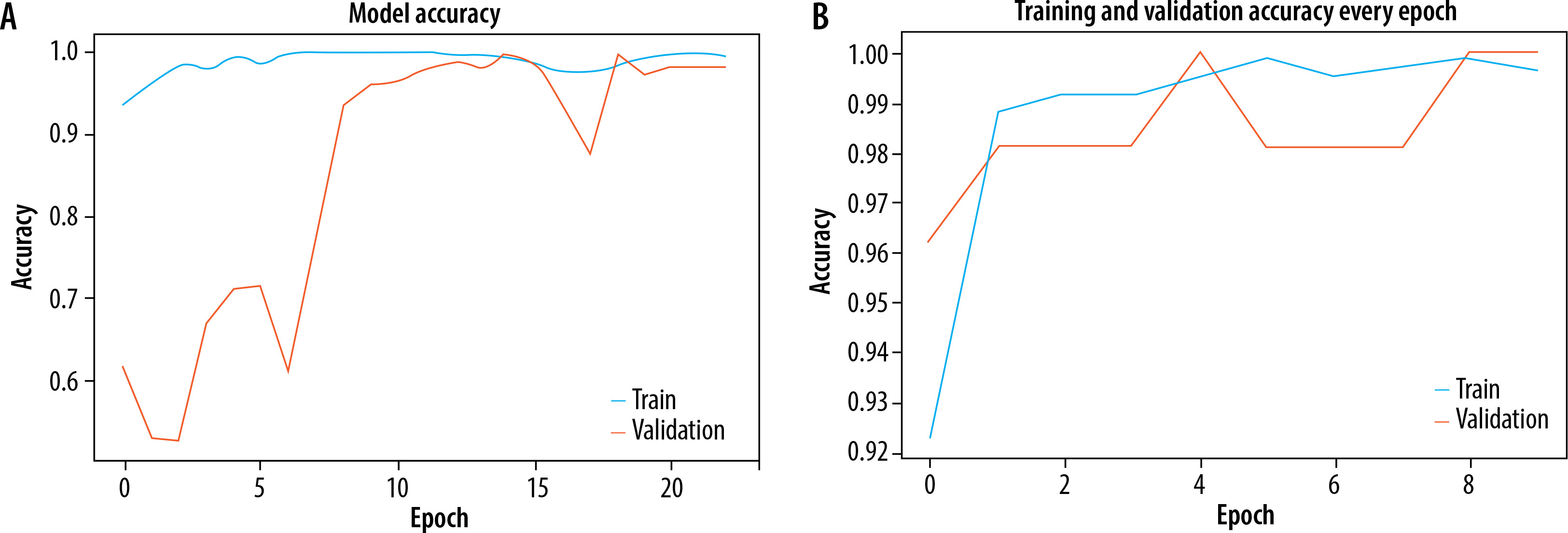
The Adam optimizer was used to dynamically adjust the learning rate throughout training and sparse categorization cross entropy was used to quantify the discrepancy between the anticipated probability and actual probabilities of the target dataset. Both models were trained for 20 epochs. EfficientNetB0 outperformed Resnet50 as an individual feature extractor. The validation procedure was further broken into two distinct steps. During the first phase, just the original image dataset was used to train pre-trained models. The models were first verified using a dataset that consisted of 20% of the whole dataset. The loss and accuracy metrics were then generated for ResNet50, with a loss of 0.0073 and an accuracy of 0.89. Similarly, for EfficientNetB0, the loss was 0.0067 and the accuracy was 0.961 during the validation process. The second part of training and validation involved using the pre-processed dataset after performing edge detection and segmentation. Both models were validated using the same ratio of training and validation datasets. The Resnet50 model computed a loss of 0.0064 and an accuracy of 0.921, while the EfficientNetB0 model achieved a loss of 0.0056 and an accuracy of 0.994. The classification report showed that the precision, recall, and f1-score for efficientNetB0 on the pre-processed dataset were 0.98, 0.97, and 0.98, respectively. Figures 5A and B displays a graph illustrating the relationship between training accuracy and validation throughout the training process for the ResNet50 model for the original dataset and pre-processed dataset respectively. Figure 6A and B displays a graph illustrating the relationship between training accuracy and validation throughout the training process for the EfficientNetB0 model for the original dataset and pre-processed dataset respectively.
Figure 5
A) Plot for training and validation accuracy for ResNet50 with original dataset. B) Plot for training and validation accuracy for ResNet50 with pre-processed dataset
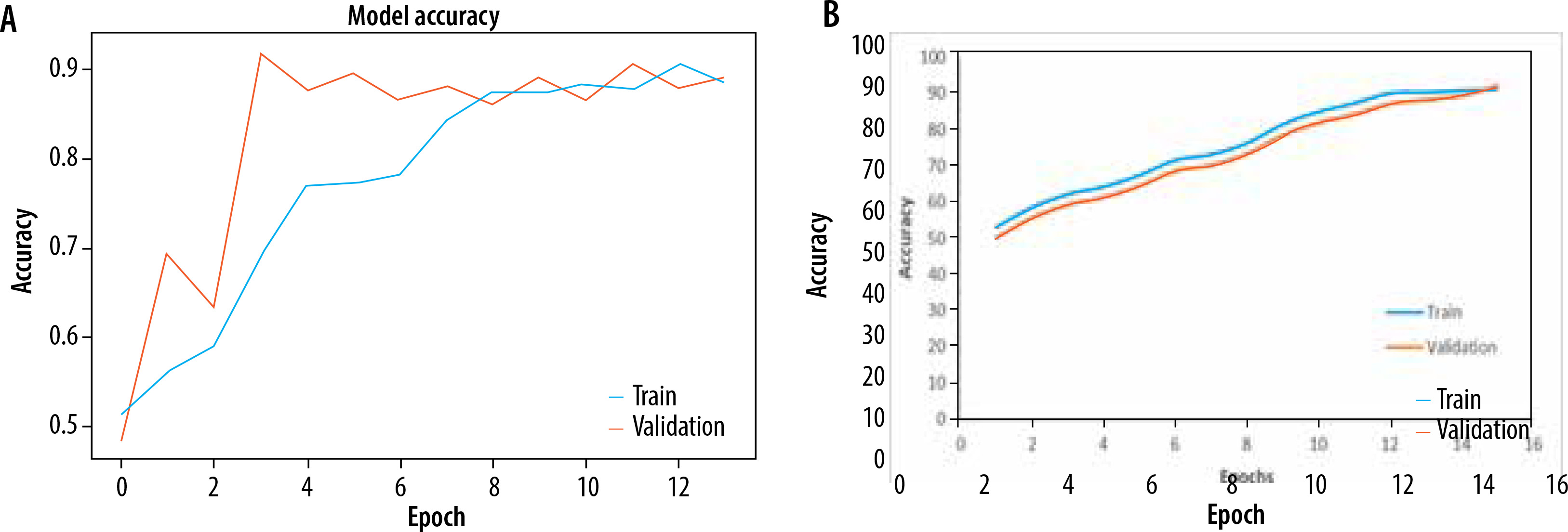
Figure 6
A) Plot for training and validation accuracy for EfficientNetB0 with original dataset. B) Plot for training and validation accuracy for EfficientNetB0 with pre-processed dataset
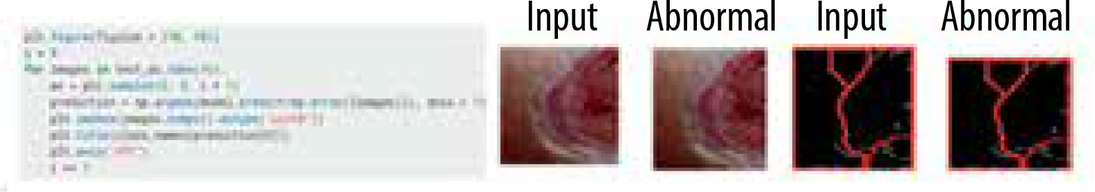
Following the completion of training and validation, the optimal model was then used to test actual photos obtained from a local physician. The process of edge detection and segmentation was performed on all the images in order to generate a pre-processed test dataset. The clinic had a total of 16 photos, with 8 being normal foot photographs and the remaining photos showing infected feet. Once a pre-processed dataset was created, the EfficientNetB0 model was evaluated using both the original collected photos and the images from the pre-processed dataset. Figure 7 displays the photos gathered from the test dataset. Figure 8 displays a portion of the code and its corresponding output.
Further, to verify the performance of the proposed model the best performing model was evaluated and compared with current state-of-the-art models [21-23]. The current models were trained using the original dataset then evaluated in the actual environment. Table 1 presents a comprehensive comparison of all the results. By examining the table, it is evident that the suggested model has strong performance in terms of accuracy and F1 score. The F1 score is a metric that may be used to measure the accuracy of a model across all classes. It takes into account both precision and recall. The classifier’s assessment is determined by its capacity to accurately recognise both positive and negative examples, which is particularly important when dealing with imbalanced classes. The suggested model, which incorporates the pre-processing steps edge detection and segmentation, outperforms all other models. Table 2 clearly demonstrates that the suggested model achieved excellent performance with the present dataset. The dataset used in our analysis is much larger than the datasets used in previous relevant studies. The majority of other models typically captured between 700 and 1000 images. Hence, based on this result, it can be said that the models exhibit diminished performance when evaluated on much bigger datasets.
Table 2
Comparison of performance metrics
| No. | Study | Method used | Test accuracy | F1 score (normal and TB class) |
|---|---|---|---|---|
| 1 | Niri et al. [21] | CNN with super pixel-based method | 0.954 | 0.89/0.92 |
| 2 | López-Cabrera et al. [22] | CNN Densenet201 without balancing | 0.921 | 0.77 / 0.91 |
| 3 | Amin et al. [23] | CNN and localization without balancing images 1055 | 0.96 | 0.91/0.90 |
| 4 | Proposed | EfficientNetB0 with original images with data balancing | 0.961 | 0.956/0.96 |
| 5 | Proposed | EfficientNetB0 with canny edge detection, watershed segmentation and data balancing | 0.994 | 0.981/0.99 |
Conclusions
The article proposes a prediction model for diabetic foot ulcer that combines deep features with hand-engineered features utilising edge detection and segmentation techniques. The model was tested in two steps. In the first phase, a model with two pre-trained networks was created to predict the original image after data augmentation. This was done to balance and increase the dataset. In the subsequent stage, the model employed canny edge detection and watershed segmentation techniques to improve performance and decrease computational expenses. Additionally, a fresh dataset was generated. The model was assessed using a Python Jupyter notebook with a dataset of 1055 photos. The dataset comprised 543 normal images while the remaining images were abnormal. Data augmentation was conducted in both stages prior to training to equalise and expand the dataset. The first step yielded a best model with an accuracy of 0.961, but the second phase produced a model with an accuracy of 0.994. The model was further evaluated in a real-time setting using random thermal images and shown to be much superior to current state-of-the-art methods. In the future, the model may be improved and rendered more authentic by including IoT devices to input patient characteristics and photos, hence enabling generation of predictions.